Easy Ways to Sum Multiple Rows and Columns in Excel: 9 Steps

If Excel had a catchphrase, it would probably be: “Please stop using a calculator for this.” One of the most common spreadsheet jobs is adding numbers across rows, down columns, or across several ranges at once. The good news is that Excel makes this wonderfully easy. The better news is that you do not need to be some mystical spreadsheet wizard who wears blue light glasses at midnight and whispers “absolute reference” into the void.

In this guide, you will learn easy ways to sum multiple rows and columns in Excel using AutoSum, the SUM function, fill handles, structured references, and a few smart tricks for real-world worksheets. Whether you are totaling sales, budgets, grades, expenses, or a suspiciously large snack spreadsheet, these methods will help you work faster and make fewer mistakes.

Let’s walk through the process in nine practical steps, with examples you can copy into your own sheet right away.

Why summing multiple rows and columns matters

At first glance, adding numbers in Excel seems almost too simple to deserve an article. Then reality arrives. Suddenly, you are summing monthly sales across six columns, calculating department totals across twenty rows, adding only filtered data, or trying to combine totals from non-adjacent ranges without accidentally including the office fantasy football tab.

That is when knowing the right Excel sum formulas pays off. A good method helps you:

• Work faster with fewer clicks
• Reduce manual errors
• Update totals automatically when data changes
• Handle adjacent and non-adjacent ranges cleanly
• Build worksheets that other humans can actually understand

Step 1: Check how your data is arranged before you sum anything

Before you use any Excel formula, look at the layout. Are your values arranged horizontally across a row, vertically down a column, or in a full table with both rows and columns? This matters because the easiest formula depends on the shape of your data.

For example, imagine this worksheet:

If you want totals for each row, you will sum across columns. If you want totals for each column, you will sum down rows. If you want everything totaled together, you may sum the whole block. Spend ten seconds checking the data orientation now, and you can save ten minutes of “Why is this number weird?” later.

Step 2: Use the status bar for a lightning-fast preview total

This method does not place a formula in your sheet, but it is perfect when you just want a quick answer. Select the cells you want to add, and Excel can show the sum on the status bar.

When to use it

• You want a fast total without changing the worksheet
• You are double-checking numbers before entering a formula
• You need a quick view of selected row or column totals

Example: highlight cells B2:E2 to preview the total for one row. Then highlight B2:B10 to preview a column total. This is the spreadsheet version of peeking at the answer key without fully committing.

Step 3: Sum one row with AutoSum

AutoSum is one of the easiest ways to add a row in Excel. Click the empty cell at the end of the row, choose AutoSum, and Excel will usually guess the range for you.

Example

If values are in cells B2:E2, click F2 and use AutoSum. Excel will typically insert:

Press Enter, and you have your row total. This is the classic “Excel does the work while you take the credit” move.

Why it works well

It is fast, beginner-friendly, and ideal when your numbers are in one clean, uninterrupted row. If the suggested range looks wrong, do not panic. Just drag to select the correct cells before pressing Enter.

Step 4: Sum one column with AutoSum

Now let’s do the same thing vertically. Click the cell below the numbers in the column and use AutoSum.

Example

If your values are in B2:B10, click B11 and Excel will usually enter:

This method is perfect for budgets, invoice lists, expense logs, and any worksheet where the numbers march politely down the page in a single file.

Pro tip

If there are blank cells or text inside the data, Excel may still work fine, but always glance at the highlighted range before hitting Enter. Blind trust is great in dog movies, less great in spreadsheets.

Step 5: Sum multiple rows or columns at the same time

This is where Excel starts to feel truly helpful. You can create several totals in one move if the rows or columns are adjacent.

How it works

Select multiple empty cells where you want totals to appear, then use AutoSum.

Example for multiple columns

If columns B, C, and D each contain numbers from row 2 to row 10, select cells B11:D11 and click AutoSum. Excel will place a separate SUM formula under each column.

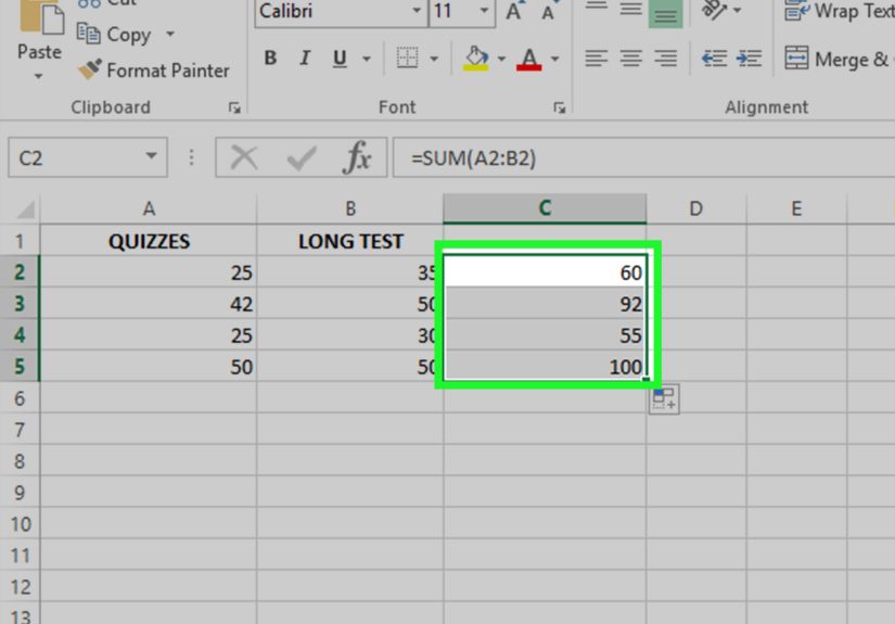
Example for multiple rows

If rows 2 through 5 each contain values across columns B:E, select cells F2:F5 and use AutoSum. Excel will add each row individually.

This is one of the easiest ways to sum multiple rows and columns in Excel because it saves time and avoids repetitive typing. It is also deeply satisfying in the way only spreadsheet efficiency can be.

Step 6: Use the SUM function for non-adjacent rows and columns

Sometimes your data is not neatly packed together. Maybe you need to total January, March, and May while skipping February and April. This is where the SUM function becomes your best friend.

Basic syntax

You can add separate cells, full ranges, or a mix of both.

Example 1: Sum non-adjacent columns

This adds values in columns B, D, and F across the same row range.

Example 2: Sum non-adjacent rows

This totals rows 2, 4, and 6 across columns B through E.

Example 3: Mix cells and ranges

This flexibility is incredibly useful when your worksheet is messy, imported from another source, or created by someone who clearly enjoys chaos.

Step 7: Copy the formula across rows or down columns with the fill handle

If you need totals for many rows or many columns, do not write the same formula over and over like it is 1997. Enter the first SUM formula, then copy it using the fill handle.

Example

In F2, enter:

Then drag the fill handle down from F2 to F20. Excel adjusts the references automatically:

You can do the same across columns. If B11 contains =SUM(B2:B10), drag right to C11, D11, and beyond.

Why this matters

This is the fastest method when you have a repeating structure, such as monthly totals for each employee, student scores by subject, or product sales by region.

Step 8: Sum by condition with SUMIF or SUMIFS

Sometimes you do not want every number. You only want totals that meet a rule. Maybe only totals for the East region, or only expenses over a certain amount, or only sales for one product line. That is where SUMIF and SUMIFS come in.

Use SUMIF for one condition

This sums values in B2:B10 only when the corresponding cell in A2:A10 equals “East.”

Use SUMIFS for multiple conditions

This totals values in C2:C20 only when the region is East and the quarter is Q1.

When it helps with rows and columns

Conditional formulas are especially helpful in larger tables where rows represent records and columns represent fields such as department, month, category, and amount. Instead of manually filtering and then guessing, you let the formula do the thinking.

Step 9: Turn your range into a table for smarter totals

If you work with growing data, convert the range into an Excel table. This makes formulas easier to read and helps totals expand automatically as new rows are added.

Why tables help

• Formulas are easier to manage
• Structured references are more readable
• Totals can update as the table grows
• Filtered data works more cleanly with subtotal tools

Example using a structured reference

That formula is much easier to understand than something like =SUM(G2:G5000), especially six months later when you have forgotten what column G was supposed to be.

Bonus idea for filtered data

If you are summing visible rows in a filtered list, consider using a subtotal-style approach instead of a regular SUM formula. A normal SUM includes hidden rows, which can lead to awkward “Why does this total hate me?” moments.

Common mistakes when summing multiple rows and columns in Excel

1. Summing the wrong range

Always check the highlighted cells before pressing Enter. AutoSum is smart, but it is not psychic.

2. Including header text by accident

Headers usually do not break the formula, but they can make the selected range look messy and confusing.

3. Forgetting that hidden rows are still included

A normal SUM formula counts hidden values unless you specifically use a method designed for filtered data.

4. Copying formulas without checking references

Most of the time relative references are helpful. Sometimes they quietly drift into the wrong columns like a shopping cart with one bad wheel.

5. Using SUMIF or SUMIFS with mismatched ranges

Make sure your criteria range and sum range line up correctly. If one starts on row 2 and the other starts on row 3, Excel may return confusing results.

Best formula examples you can reuse

Here are several practical Excel formulas for summing multiple rows and columns:

These cover most everyday situations, from simple row totals to more advanced multi-criteria reporting.

Real-world examples of summing rows and columns

Monthly budget tracker

Each row is a category like rent, groceries, utilities, and entertainment. Each column is a month. Use row totals to see category spending and column totals to see monthly spending.

Sales report

Each row is a sales rep. Each column is a product or month. Sum rows to measure rep performance, and sum columns to compare product or monthly totals.

Grade book

Each row is a student and each column is an assignment. Total rows for final points and total columns to compare assignment performance.

Inventory sheet

Each row is an item, while columns track quantities in different warehouses. Sum across a row to get total stock per item, or down a column to see stock per location.

Experience-based tips: what people usually learn the hard way

The funny thing about Excel is that most people do not really learn it in a class. They learn it in the wild. Usually under pressure. Usually while trying to finish a report before lunch, before payroll, before a meeting, or before someone from accounting sends the dreaded “just checking in” email.

One of the first real experiences many people have with summing multiple rows and columns is realizing that there is a huge difference between “I got a number” and “I got the right number.” That sounds obvious, but it is the spreadsheet version of discovering that just because the car starts does not mean you should drive it across the country. A total that looks reasonable can still be wrong if one row was skipped, one extra column was included, or one hidden section stayed inside the formula like an uninvited guest.

Another common experience is starting out with manual addition. People click cells one by one, build heroic little formulas, and then repeat the process for ten more rows. At first it feels productive. Then they discover AutoSum, the fill handle, or a simple SUM formula copied down the page, and suddenly they realize they have been doing spreadsheet cardio for no reason. That moment is part relief, part annoyance, and part “Where has this been all my life?”

People also learn quickly that clean layouts make summing much easier. When a worksheet is organized consistently, with clear headers and uninterrupted data ranges, Excel behaves like a helpful assistant. When the sheet has random blank columns, merged cells, decorative formatting experiments, and totals jammed in the middle of raw data, Excel behaves more like a confused intern on day one. A lot of experience with Excel is really experience with designing data so formulas stay simple.

Then there is the classic filtered-data surprise. Someone filters a table, sees only five visible rows, and assumes the total reflects only what is on the screen. But a regular SUM formula may still include hidden rows. That can be a memorable lesson, especially when the total is used in a meeting and another person politely asks why the “visible” subtotal appears to include values from places nobody can currently see. After one or two moments like that, users become much more careful about which total method they choose.

Experienced Excel users also become protective of readability. Yes, you can write a giant formula that snakes across multiple ranges and conditions like a spreadsheet octopus. But should you? Usually not. Over time, people learn that the best formulas are the ones they can still understand later. Simple SUM ranges, consistent references, and table-based formulas save enormous amounts of time when a workbook needs to be updated or handed to someone else.

Perhaps the most useful experience of all is realizing that Excel rewards small habits. Check the range. Label the totals. Copy formulas instead of retyping them. Test one row before filling twenty. Keep your structure consistent. These are not glamorous skills, but they prevent the kind of errors that create long afternoons and awkward explanations. In other words, the real Excel superpower is not dramatic formula wizardry. It is being boring in exactly the right places.

Conclusion

If you need to sum multiple rows and columns in Excel, the easiest method depends on the job in front of you. AutoSum is fantastic for quick adjacent totals. The SUM function is ideal for custom ranges and non-adjacent data. Fill handles make repeated totals painless. SUMIF and SUMIFS help when conditions matter. And tables make everything more scalable and readable as your worksheet grows.

The key is not memorizing every possible formula. It is knowing which tool fits the moment. Once you understand these nine steps, you can total rows, columns, and whole data sets much faster, with far less frustration and a significantly lower chance of shouting at your monitor.

SEO Tags